Text lets an incorrect explanation remain elegant. A simulation is less polite. The bridge falls, the orbit escapes, or the ball passes through the floor.
I wanted to test a narrow version of a larger idea:
Can a model with fewer than one billion parameters learn enough structured code to generate small interactive physics worlds?
The repository contains a completed Qwen3 0.6B LoRA run built from synthetic p5.js examples. It also contains a developmental learning proposal for MuJoCo. One asks a model to write worlds. The other asks a model to learn inside them. The completed training run gives us a useful first measurement.
Experimental setup
One hundred parallel Claude agents generated examples across 124 school science topics. The resulting curriculum covered mechanics, electricity, waves, thermodynamics, fluids, optics, astronomy, chemistry, and biology.
| Component | Value |
|---|---|
| Base model | Qwen3 0.6B |
| Trainable parameters | 40.4M |
| Share of model trained | 5.1% |
| LoRA rank | 64 |
| LoRA alpha | 128 |
| Hardware | 4 A100 GPUs |
| Effective batch size | 32 |
| Training time | 171.87 seconds |
Every target followed the same executable grammar: a canvas, setup(), draw(), state variables, and visible consequences over time.
function draw() {
  velocity.add(gravity);
  position.add(velocity);

  if (position.y > floorY) {
    position.y = floorY;
    velocity.y *= -restitution;
  }
}
This pattern is small, but it contains a causal claim. Gravity changes velocity. Velocity changes position. Collision reverses and damps motion.
Training curve
| Step | Loss | Token accuracy |
|---|---|---|
| 10 | 0.909 | 77.0% |
| 30 | 0.621 | 82.3% |
| 50 | 0.549 | 84.0% |
| 70 | 0.510 | 84.9% |
| 93 | 0.592 | 85.6% |
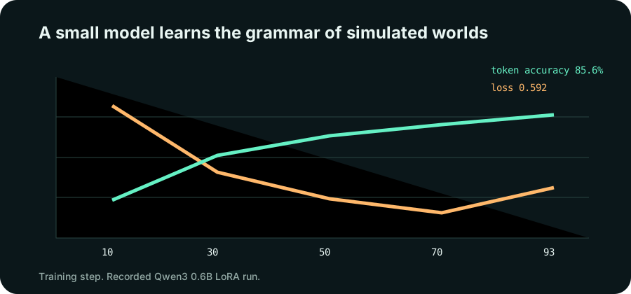
Token accuracy rose 8.6 points while loss fell rapidly. The final loss rose above the step 70 value, so the clean story is not “training improved forever.” The better reading is that the model found the domain grammar quickly and then entered a noisier regime near the end.
Training completed in 2.9 minutes. That is the first persuasive result. A narrow visual programming language can be distilled into a small model cheaply enough to iterate.
New run: does the generated integrator preserve the law?
Token accuracy cannot detect a numerically unstable world. I added a deterministic benchmark for the harmonic oscillator, x'' = -x, and ran each method for 20 simulated seconds. The reference solution is x(t) = cos(t), and the invariant is total energy E = 0.5(x² + v²).
| Integrator | dt | Steps | Final energy drift | Maximum drift | Final position error |
|---|---|---|---|---|---|
| Explicit Euler | 0.10 | 200 | 631.60% | 631.60% | 0.8568 |
| Semi implicit Euler | 0.10 | 200 | 3.25% | 5.26% | 0.0535 |
| Velocity Verlet | 0.10 | 200 | 0.21% | 0.25% | 0.0076 |
| Velocity Verlet | 0.05 | 400 | 0.052% | 0.062% | 0.0019 |
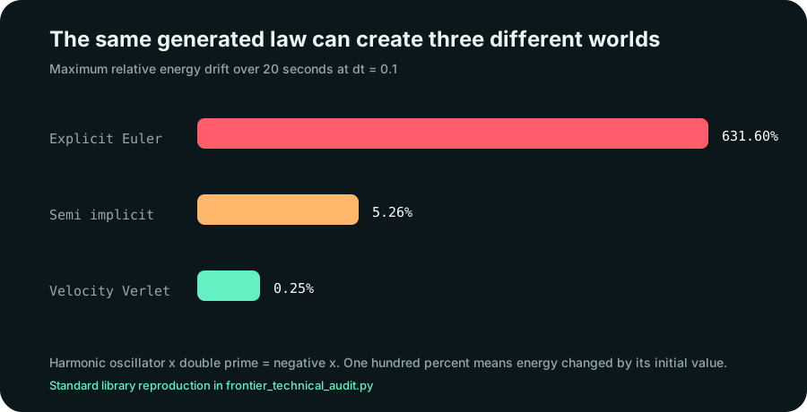
The explicit update diverged even though every line of code was syntactically reasonable. At the same time step, Velocity Verlet reduced maximum energy drift by roughly 2,527 times. This is why an execution benchmark must score invariants rather than screenshots.
The experiment is reproducible with no third party packages:
python experiment-tools/frontier_technical_audit.py `
  --output experiment-tools/results/frontier_technical_audit.json
The generated JSON records the time step, number of integration steps, maximum energy drift, final energy drift, and phase error for all nine method and step size combinations.
Change gravity and surface drag above. A parameter change produces a visible consequence. That immediate feedback is the reason simulated worlds are more than decorative output.
Why token accuracy is not enough
An 85.6 percent next token score does not mean 85.6 percent of generated simulations are physically correct. One wrong operator can create energy from nowhere. A missing boundary condition can invalidate an otherwise perfect file.
The next evaluation should therefore execute the output and score behavior.
def score_trajectory(predicted, reference):
    position_error = mean_distance(predicted.xy, reference.xy)
    energy_drift = abs(predicted.energy[-1] - reference.energy[-1])
    runtime_ok = int(predicted.completed_without_error)
    return runtime_ok, position_error, energy_drift
I would use at least four metrics:
| Metric | What it catches |
|---|---|
| Runtime pass rate | Invalid JavaScript |
| Trajectory error | Wrong motion |
| Energy drift | Physically impossible behavior |
| Teacher rating | Misleading explanation |
A production harness should parse the emitted JavaScript, execute it in a time limited browser worker, sample state on every frame, and compare invariant traces. For a pendulum, measure energy and period. For a projectile, measure acceleration and range. For a collision, measure momentum and restitution. The evaluator should never depend on one visual snapshot.
def invariant_score(trace, invariant):
    expected = invariant(trace[0])
    relative_drift = [abs(invariant(s) - expected) / max(abs(expected), 1e-9)
                      for s in trace]
    return {
        "max_drift": max(relative_drift),
        "p95_drift": percentile(relative_drift, 0.95),
        "stable": all(math.isfinite(x) for state in trace for x in state),
    }
The teacher rating matters because correct motion can still teach badly. Labels can cover the important object. Time can move too quickly. A beautiful animation can emphasize the wrong variable.
The failure that points forward
The final loss wobble and the gap between token accuracy and executable truth lead to the same conclusion. Static language metrics are a first filter, not the destination.
The exciting loop is closed:
A model predicts a world.
The world runs.
Its trajectory is compared with the intended law.
The failure becomes the next training example.
This is how a simulator begins to teach back. The model is no longer rewarded only for resembling code in the archive. It is rewarded for creating a world that survives contact with its own rules.
The experiment supports a modest claim with large consequences. Small models can acquire the grammar of interactive scientific explanation quickly. The remaining frontier is not more fluent code. It is automatic contact with reality, even if that reality is only 600 pixels wide.
Reproduction and provenance
The training curve is transcribed from the committed p5.js experiment report. The integrator benchmark is newly executed standard library code. Run python experiment-tools/frontier_technical_audit.py from the repository root. The generated JSON contains every unrounded value used in the table.