What if a model did not reread its past in words?
That question led to the largest completed experiment in this repository: compress long documents into latent vectors, project those vectors into soft tokens, and compare the result with a text summary buffer.
The experiment began with an attractive hypothesis:
Latent Pager Memory can preserve useful information with less generation cost than a text buffer.
The data supported that hypothesis and exposed a dangerous price.
Architecture
The text baseline chunks a document, generates a summary for each chunk, concatenates the summaries, and generates an answer. The latent pager replaces the summaries with hidden state extraction and learned soft tokens.
hidden = frozen_model(chunk, output_hidden_states=True).hidden_states[-1]
page = compressor(hidden[-1])
soft_tokens = aggregator(page, num_tokens=16)
answer = frozen_model.generate(inputs_embeds=soft_tokens)
The final model used last token pooling, 16 soft tokens, and one aggregator layer. It was trained on 2,000 examples and tested on 500 examples covering single fact extraction and multi hop reasoning.
In tensor terms, the frozen transformer emits hidden states H ∈ R^(L × d_model). Last token pooling selects h_L. A learned compressor maps that vector into d_page, and an aggregator expands the page representation into k soft tokens S ∈ R^(k × d_model). Those tokens enter the frozen decoder through inputs_embeds.
tokens -> frozen transformer -> h_L -> compressor -> page vector
page vector + learned queries -> aggregator -> k soft tokens -> decoder
Increasing k increases the activation bandwidth and the aggregator parameter surface. The ablation is therefore not merely “more memory slots.” It changes capacity, optimization, and the number of continuous prompt vectors the decoder can exploit.
Main result
| Metric | Text buffer | Latent pager | Change |
|---|---|---|---|
| F1 | 0.0182 | 0.0257 | +41.5% |
| ROUGE L | 0.0177 | 0.0260 | +47.0% |
| Average latency | 19.55 s | 7.65 s | 2.55 times faster |
| Peak memory | 1.02 GB | 1.82 GB | +77% |
| Hallucination | 0.292 | 0.580 | +98.4% |
All paired quality differences were reported significant at p less than 0.001 using 10,000 bootstrap iterations.
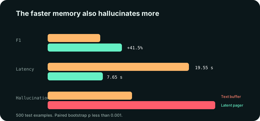
The latent pager was faster and closer to the reference answer. It also hallucinated almost twice as often.
That is the real experiment. If I reported only F1 and latency, the method would look like a clean win. Adding hallucination turns the result into a design problem.
Conceptual view based on the direction of the recorded context stress results. This is not a new benchmark.
The interactive landscape above is conceptual. The table is measured. Keeping those categories separate matters because an appealing visualization can otherwise lend certainty to data it did not produce.
Task breakdown
| Task | Text F1 | Latent F1 | Text hallucination | Latent hallucination |
|---|---|---|---|---|
| Single fact, 260 tests | 0.0206 | 0.0314 | 0.317 | 0.662 |
| Multi hop, 240 tests | 0.0155 | 0.0195 | 0.265 | 0.491 |
Compression helped single fact retrieval more than multi hop reasoning. That makes architectural sense. A compressed page can preserve a local signal while still losing the relationships needed to combine facts across chunks.
The single fact hallucination rate of 0.662 is the loudest warning. The representation gave the decoder enough semantic scent to answer, but not always enough evidence to answer faithfully.
Three versions, two wrong turns
| Version | Design | Test F1 |
|---|---|---|
| 1 | Mean pooling, 32 tokens, 2 layers | 0.0136 |
| 2 | Question conditioning plus reconstruction loss | 0.0143 |
| 3 | Last token, 16 tokens, 1 layer | 0.0257 |
Version one underperformed the text baseline. Version two added clever machinery and barely improved. Version three removed machinery and won.
The ablations explain why.
| Ablation | F1 | Hallucination |
|---|---|---|
| Mean pooling | 0.0191 | 0.273 |
| Last token pooling | 0.0231 | 0.073 |
| 8 soft tokens | 0.0186 | 0.211 |
| 16 soft tokens | 0.0240 | 0.271 |
| 64 soft tokens | 0.0171 | 0.316 |
Last token pooling improved F1 by 21 percent over mean pooling and reduced hallucination by 73 percent in that ablation. Sixteen soft tokens formed the quality peak. More capacity did not mean more memory. It meant more parameters available to overfit.
Pareto frontier and decision boundary
I encoded the recorded soft token ablations and computed nondominance using higher F1 and lower hallucination as the two objectives.
| Tokens | F1 | Hallucination | Pareto status |
|---|---|---|---|
| 8 | 0.0186 | 0.211 | Nondominated |
| 16 | 0.0240 | 0.271 | Nondominated |
| 32 | 0.0191 | 0.273 | Dominated by 16 |
| 64 | 0.0171 | 0.316 | Dominated by 8 and 16 |
| 128 | 0.0163 | 0.261 | Dominated by 8 |
Only 8 and 16 tokens survive. Sixteen is the quality operating point. Eight is the caution operating point. Reporting only the maximum F1 would hide that product decision.
The main comparison can be expressed as a utility function:
U = F1 - lambda_h * hallucination - lambda_t * latency

Delta U for latent minus text
  = 0.0075 - 0.288 * lambda_h + 11.90 * lambda_t
If latency has zero weight, the text buffer becomes preferable when lambda_h > 0.02604. In other words, assigning a penalty of only 0.026 F1 units to a full unit of hallucination erases the latent pager’s quality advantage. If latency matters, its 11.9 second advantage pushes the decision boundary back toward the latent method.
This equation makes the engineering choice explicit. There is no universal winner without a cost model.
The experiment I would run next
The decoder needs permission to abstain. I would add a retrieval sufficiency head trained to predict whether the latent pages contain enough evidence.
evidence_score = sigmoid(sufficiency_head(soft_tokens.mean(0)))

if evidence_score < threshold:
    return "I do not have enough evidence in memory."
return decoder.generate(soft_tokens)
The evaluation should plot F1 against hallucination as the threshold changes. The goal is not maximum recall. It is a useful operating point where compression gains survive without doubling fabricated answers.
The correct summary statistic is a risk coverage curve. Sort examples by sufficiency score, answer only the top fraction, and plot hallucination risk against coverage. The area under that curve allows two abstention heads to be compared without choosing a deployment threshold in advance.
The repository does not include the 500 per example memory outputs, so the utility and Pareto audit above reproduces calculations from the committed aggregate tables rather than pretending to rerun bootstrap inference. The technical audit JSON labels those values as recorded_main_result for that reason.
What the data convinced me of
Latent memory is not merely a smaller cabinet. It changes the failure mode. Text summaries can omit. Latent vectors can suggest. Suggestion is powerful because it is fast and associative. It is dangerous because a decoder can turn a faint association into a confident sentence.
The uncharted path is real. The experiment shows a 2.55 times speed advantage and a 41.5 percent F1 improvement. It also places a warning sign at the entrance: memory quality must include knowing when the memory is insufficient.
When memory becomes a place, the system needs more than a path back. It needs landmarks that distinguish what was truly there from what merely feels familiar.
Reproduction and provenance
Run python experiment-tools/frontier_technical_audit.py to rebuild the Pareto frontier and utility boundary. The raw 500 example memory outputs are not committed here, so F1, latency, hallucination, and bootstrap significance remain traceable recorded aggregates rather than falsely reproduced row statistics.