A company or a country is sometimes talked about as one living system. That metaphor was the question. The sources below do not support it.
The practical question is how to initialize a swarm. For a fixed group of 48 agents, what mix of roles should you start with? Who specializes, who stays broad, who coordinates, who communicates, and how do you promote, if the score is either discovery or revenue?
Two failure modes are worth designing against. One is too many cooks: the links among people grow faster than the coordination skill on hand. The other is a mass of people idle: headcount that is present and not producing.
No source that was opened gives an 80% idle law. Pareto’s income curve is not the claim that 20% of employees do 80% of the work.
The simulation is in agent-org-forms. It is a design you can run. It is not an estimate of the right manager fraction in a real firm.
What the sources actually support
Span of control is a load problem: Nickols reconstructs Graicunas as a relationship count of 44 at 4 subordinates, 100 at 5, and 222 at 6, from \(n(2^{n-1}+n-1)\), quotes Hamilton’s rule of thumb as groups of about three near the top and about six near the bottom, and reports Urwick’s point that a span that is too wide costs indecision and bad communication, a cost that has to be weighed against extra managers (Nickols).
Gittell’s Organization Science 2001 abstract says smaller supervisory spans raised airline departure performance through relational coordination (RePEc).
Cheon 2022, in the Journal of Policy Studies, looks at 101 Korean quasi-governmental organizations and finds a wider top span associated with government performance scores (beta 0.055), a wider mid span negatively associated (beta -1.209, and the mid-span variable was divided by 1000, so that is not per extra employee), and no significant link from span to customer satisfaction (Journal of Policy Studies).
Garvin, in Harvard Business Review in December 2013, reports that a 2002 no-manager experiment at Google lasted a few months, and that some engineering managers were given about 30 reports so they could not micromanage (Harvard Business Review).
Project Oxygen, on the re:Work page, says teams with higher-rated managers had better results, satisfaction, and lower turnover, and that effective sales teams beat target by 17% on average while ineffective ones missed by up to 19%; that is company research, not a journal estimate of the right fraction of managers (re:Work).
March 1991, in Organization Science, argues that exploration and exploitation are both required, that fast socialization raises short-run knowledge and cuts diversity, and that a mix of fast and slow learners beat a homogeneous group on equilibrium knowledge (March 1991).
The Teodoridis, Bikard, and Vakili SSRN abstract says generalists did better when the pace of change was slow and specialists gained when it sped up (SSRN).
The Teodoridis Kinect abstract says that when a tool got cheap, generalists substituted for area specialists; the full papers were not opened (SSRN).
Brooks, in The Mythical Man-Month, treats training as linear in headcount and pairwise communication as \(n(n-1)/2\) (Mythical Man-Month).
Latané, Williams, and Harkins 1979 separate social loafing from coordination loss, cite Ringelmann via Moede as a solo rope pull of 63 kg, three people at 160 kg, and eight people at 248 kg (eight people produced 49% of the sum of solos), and still find loafing in a shouting experiment with coordination removed, where a power of about -0.14 fit 93% of the variance in that one task, an exponent that is not a universal constant (Latané, Williams, and Harkins).
Benson, Li, and Shue, in the Quarterly Journal of Economics, find that in 131 firms higher pre-promotion sales raised promotion chance and predicted lower manager value added, that a doubling of pre-promotion sales lined up with about a 6.1% drop in each subordinate’s sales, and that a counterfactual which promoted on predicted managerial quality had about 30% higher average manager value added; they do not call this a proven mistake, the incentive value may be worth it, and collaboration experience predicted better managing (Benson, Li, and Shue).
Lazear and Rosen 1981 show that a rank-order prize can induce the same effort as a piece rate (Lazear and Rosen).
Coase 1937 argues that a firm should stop growing when the cost of one more internal transaction equals the market, which is not a superorganism (Coase).
Simon 1962 argues that complex systems are usually hierarchies of subsystems, that nearly decomposable structure evolves faster, and that the real organization is not the paper org chart (Simon).
Dunbar 1993 reports that a primate regression predicts a human group size of 147.8, with a 95% interval from 100.2 to 231.1, an extrapolation outside the data, and treats that figure as a claimed limit on a cohesive personal network, not a management span (Dunbar).
Persky 1992 states Pareto’s result as an income curve \(\log N = A - \alpha \log x\), with alpha near 1.5, and notes that at alpha 1.5 the top 20% of recipients got about 58% of income, not 80% (Persky).
Larson 2018 is a practitioner rule, not a study: 6 to 8 engineers per manager (Larson).
Reddit threads were not opened, after timeouts, and nothing here is taken from them.
These were not opened: Meier and Bohte 2000, Theobald and Nicholson-Crotty 2005, Graicunas 1933 itself, Peter and Hull’s book, Steiner 1972, Ringelmann 1913, the Teodoridis full texts, and Price’s 1963 book.
The model
The file is simulate.py. The equations below are the ones that file runs.
Roles sit on a simplex. The script calls the specialist share of the maker pool specialist_share. Writing that share as \(s_{\mathrm{spec}}\),
$$ \pi_S + \pi_G + \pi_C + \pi_K = 1, $$$$ \pi_S = s_{\mathrm{spec}}(1 - \pi_C - \pi_K), \qquad \pi_G = (1 - s_{\mathrm{spec}})(1 - \pi_C - \pi_K). $$Integer counts are the largest-remainder split of \(\pi N\), with \(N = 48\). Every seed in a cell gets the same counts.
A trait vector is \(\theta = (d, b, c, k, a)\): depth, breadth, coordination skill, communication skill, and a scale on making. The code draws
$$ \theta = \mathrm{sigmoid}(\mu_{\mathrm{role}} + \varepsilon), \qquad \varepsilon \sim \mathcal{N}(0, \sigma^2 I), $$$$ \mathrm{sigmoid}(x) = \frac{1}{1 + \exp(-x)}. $$The logit prototypes \((d, b, c, k, a)\) are \((2, -1, -1, 0, 0)\) for a specialist, \((0, 2, -0.5, 0.5, 0)\) for a generalist, \((-0.5, 0, 2, 0.5, 0)\) for a coordinator, and \((-1, 0.5, 0, 2, 0)\) for a communicator. On the main grid, \(\sigma = 0.5\).
Specialty \(s\) is a distribution on \(K = 8\) domains. Specialists use a Dirichlet draw with concentration 20 on one random domain and 0.4 elsewhere. Everyone else uses a symmetric Dirichlet with concentration 1. Normalized entropy is
$$ H(s) = \frac{-\sum_j s_j \log s_j}{\log K}. $$Time runs for \(T = 200\) periods. A shock at \(t = 100\) sets \(z_t = 0\) before the shock and \(z_t = 1\) at and after it. There is no partial mix. Making uses breadth before the shock and depth after it:
$$ m_i = a_i \, b_i \, (1 - H(s_i)) \quad \text{if } z_t = 0, $$$$ m_i = a_i \, d_i \, (s_i \cdot q_t) \quad \text{if } z_t = 1. $$Production uses true specialty \(s\), not belief. Team making is the sum of \(m\) over members of the team,
$$ P = \sum_i m_i. $$Period load \(\lambda_t\) is 0.2 on even \(t\) and 0.8 on odd \(t\). Each seed-period is sparse with probability 0.5, on two random domains; otherwise the task \(q_t\) is a Dirichlet draw. At and after the shock, a seed-specific permutation moves that task mass.
Brooks loss inside a team of size \(n\) is the pairwise term, scaled by that period’s load. The main loop does not use the Graicunas count. The code’s loss is
$$ L = \lambda_t \, \frac{n(n-1)}{2}. $$Coordinator skill in the team is \(S_C\), the sum of \(c\) over coordinators. The gap and the factor are
$$ g = \max(0, L - S_C), \qquad \mathrm{factor} = \exp\left(-\alpha \frac{g}{L+1}\right). $$If \(L = 0\), the factor is 1. Extra coordinator skill past \(L\) does not raise the factor.
Loafing is not a separate draw \(e_i\). The code sets one effort for every member of a block. Let \(\bar{c} = S_C / n\), and let \(\bar{k}\) be the mean communicator skill \(k\) in the block, or 0 if the block has no communicator. With the unfitted weights \(\eta_C = \eta_K = 2\),
$$ \rho = \mathrm{sigmoid}(2\bar{c} + 2\bar{k}), \qquad e = \rho + (1-\rho)\, n^{\gamma}. $$Block output before any cross term is \(P\) times \(e\) times the factor.
Three structures use the same people. Flat is one group of 48, so \(n = 48\) and there is no cross-block term. Modules are six blocks of 8. Within each block, \(L\) still uses \(\lambda_t\). The cross-block load is a small constant, not scaled by \(\lambda_t\):
$$ L_{\mathrm{cross}} = 0.05 \cdot \frac{6 \cdot 5}{2} = 0.75. $$Surplus coordinator skill after within-block demand, \(S_{\mathrm{cross}}\), can offset that load:
$$ g_{\mathrm{cross}} = \max(0, L_{\mathrm{cross}} - S_{\mathrm{cross}}), \qquad f_{\mathrm{cross}} = \exp\left(-\alpha \frac{g_{\mathrm{cross}}}{L_{\mathrm{cross}}+1}\right). $$Organization output is
$$ Y = f_{\mathrm{cross}} \sum_b (P_b \, e_b \, \mathrm{factor}_b). $$Isolated modules are the same blocks with the cross-block term set to 0, so \(f_{\mathrm{cross}} = 1\). That switch is a design choice. It is not a measurement.
Agreement \(u\) is the fraction of makers whose argmax belief equals the argmax of the organizational code, measured before the update. If there are no makers, \(u = 0\). This update is not March’s recursion. The organizational code starts uniform, and belief starts at \(s\). Makers whose specialty matches the task better than the code pull the code. Communicators pull maker beliefs toward the code. In the formulas, mean_a is the mean of \(a\) among those better-matching makers, or 0 if there are none, and mean_k is the mean communicator skill \(k\), or 0 if there are no communicators:
$$ p_2 = 0.05 + 0.2 \cdot \mathrm{mean\_a}, \qquad p_1 = 0.02 + 0.5 \cdot \mathrm{mean\_k}. $$The vote is making-weighted specialty among makers, and then
$$ \mathrm{code} \leftarrow \mathrm{normalize}\bigl((1-p_2)\,\mathrm{code} + p_2 \,\mathrm{vote}\bigr), $$$$ \mathrm{belief} \leftarrow (1-p_1)\,\mathrm{belief} + p_1 \,\mathrm{code} $$for every maker.
Discovery and revenue split by the shock and by agreement. Primary scores use \(Y\), not a net that penalizes idle share:
$$ D_t = Y_t \, z_t \, (1 - u_t), \qquad R_t = Y_t \, (1 - z_t) \, u_t. $$So cumulative revenue is entirely pre-shock, because \(R_t = 0\) for \(t \ge 100\), and cumulative discovery is entirely post-shock, because \(D_t = 0\) for \(t < 100\).
Idle is a count. Coordinator idle mass in a block is \((S_C - L)/S_C\) times the number of coordinators when \(S_C > L\), and 0 otherwise. On modules, surplus used to cover \(L_{\mathrm{cross}}\) is not idle. A maker is idle when \(e \cdot m\) is strictly below half the median of \(e \cdot m\) among makers. The 10th percentile is not the threshold. Then
$$ \iota = \frac{\text{idle coordinator mass} + \text{idle makers}}{N}. $$A side score, not the one used for \(D\) and \(R\), is
$$ Y_{\mathrm{net}} = Y \bigl(1 - \max(0, \iota - \iota_0)\bigr). $$\(\iota_0\) is a scenario knob. It is 0.5 in this run. The value 0.8 was only a failure check on the within-run median of \(\iota\). It was not a target inside the score.
Promotion, on the extra cells only, happens at \(t = 80\), before production. Peter promotes the 4 makers with the largest depth \(d\). Match promotes the 4 makers with the largest breadth \(b\). Both then set the new coordination skill from depth and breadth and zero the maker depth:
$$ c \leftarrow \mathrm{sigmoid}(\beta_0 + \beta_1 d + \beta_2 b), $$with \(\beta_0 = 0\) and \(\beta_2 = 1\) in the code, then \(d \leftarrow 0\) and the role becomes coordinator. Tournament does not change roles. The top quartile of makers, by mean \(m\) over the previous 10 periods, gets 0.15 added to \(\mathrm{logit}(a)\). That quartile stands in for a prize. It is not a random draw.
The main grid is \(N = 48\), \(K = 8\), \(T = 200\), shock at \(t = 100\), and 30 seeds. Coordinator share is in \(\{0, 0.0625, 0.125, 0.25, 0.5\}\), specialist share of the maker pool is in \(\{0.25, 0.5, 0.75\}\), and communicator share is in \(\{0, 0.1\}\). Defaults are \(\alpha = 1\), \(\gamma = -0.14\), and \(\sigma = 0.5\). The promotion comparison moves 4 agents at \(t = 80\). A sweep uses \(\alpha \in \{0.5, 1, 2\}\) and \(\gamma \in \{0, -0.14, -0.5\}\), 10 seeds, modules only, and \(\beta_1 \in \{-1, 0, +1\}\) on the promotion cells.
\(\alpha\), \(\gamma\), \(\sigma\), \(\beta_1\), and \(\iota_0\) are free design choices. They are not fitted constants. Every ± below is the sample standard deviation across seeds, with the usual \(n-1\) denominator. The main grid uses 30 seeds. The sweeps use 10.
Results
On the plotted slice, modules with specialist share 0.5 and communicator share 0.1, cumulative revenue does not make an inverse-U in coordinator share. The five means are 97.8542 ± 5.7335, 100.4960 ± 6.4454, 96.6813 ± 8.1965, 104.4592 ± 6.8621, and 108.9716 ± 10.2031. The peak is at coordinator share 0.5.
High-lambda cumulative discovery on that same slice peaks at coordinator share 0, at 4.4015 ± 1.6868. High-lambda cumulative revenue peaks at 0.0625, at 46.5997 ± 3.0175. Flat, on the same specialist share and communicator share, peaks at coordinator share 0 for both cumulative revenue and cumulative discovery.
Isolated modules, which set the cross-block term to 0, score higher than both of the other structures on that slice. At coordinator share 0.5 the isolated cumulative revenue is 161.2728 ± 12.5979. The cross-block penalty is a design choice, so “modules beat flat” is not a result of this run. At coordinator share 0.5, specialist share 0.5, and communicator share 0.1, modules have cumulative revenue 108.9716 ± 10.2031 and flat has 110.0627 ± 7.9821.
Flat at coordinator share 0.5 is the worst cell on its slice for both metrics. That loss is not a worse Brooks gap and it is not more loafing. Coordination loss is lower than at coordinator share 0, and mean effort \(e\) is higher. At coordinator share 0, cumulative revenue is 138.3262 ± 7.9943 and mean effort is 0.9370 ± 2.5651e-03. At coordinator share 0.5, cumulative revenue is 110.0627 ± 7.9821 and mean effort is 0.9714 ± 1.7608e-03. Mean coordination loss moves from 0.6311 ± 1.1292e-16 to 0.6090 ± 3.2049e-04.
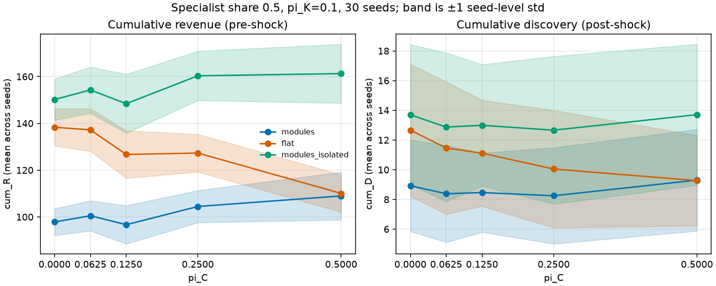
Cumulative discovery and revenue are plotted against coordinator share for a flat group, for modules, and for modules with the cross-block term removed.
Across the modules grid, the highest mean cumulative revenue is coordinator share 0.5, specialist share 0.75, and communicator share 0.1. The counts are 14 specialists, 5 generalists, 24 coordinators, and 5 communicators. Cumulative revenue is 113.8151 ± 12.0336 and cumulative discovery is 8.8004 ± 3.8421.
The highest mean cumulative discovery on modules is a different cell: coordinator share 0.25, specialist share 0.75, and communicator share 0, which is 27 specialists, 9 generalists, 12 coordinators, and no communicators. Cumulative discovery is 36.7658 ± 9.7684 and cumulative revenue is 30.2240 ± 9.9102. Revenue and discovery do not pick the same mix.
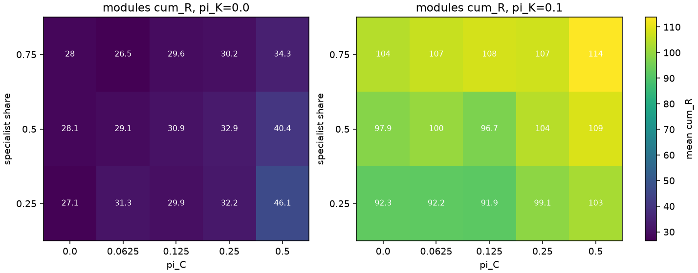
The heatmap is cumulative revenue on modules, across coordinator share, specialist share, and communicator share.
Raising communicator share from 0 to 0.1 raised cumulative revenue and lowered cumulative discovery in 15 of 15 modules cells. At coordinator share 0.125 and specialist share 0.5, cumulative revenue is 96.6813 ± 8.1965 with communicators and 30.9024 ± 6.1504 without them, while cumulative discovery is 8.4622 ± 2.6666 with them and 26.7826 ± 6.9304 without them. Agreement moves with that switch: mean pre-shock agreement is 0.9575 ± 8.2146e-03 versus 0.3046 ± 0.0575, and mean post-shock agreement is 0.8293 ± 0.0541 versus 0.4639 ± 0.1381. That is the March-shaped communicator effect in this model. Fast agreement raises pre-shock revenue and cuts post-shock discovery. Cumulative revenue is entirely pre-shock, and cumulative discovery is entirely post-shock.
The median idle share never reached 0.8. That happened in 0 of 2700 cell-seed runs. The maximum within-run median was 0.2500, on modules at coordinator share 0.0625, specialist share 0.25, and communicator share 0. The 80% idle organization was not produced by this grid, including coordinator share 0.5 inside one group of 48.
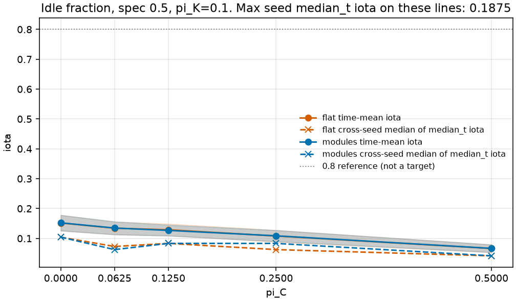
Time-mean idle share, and the cross-seed median of the within-run median, are plotted against coordinator share for the flat group and for modules.
After the shock, specialist-heavy mixes beat generalist-heavy mixes on cumulative discovery in 5 of 5 coordinator-share cells, at both communicator shares. Here specialist-heavy means specialist share 0.75 and generalist-heavy means 0.25. Before the shock, generalist-heavy beat specialist-heavy on cumulative revenue in 4 of 5 cells only when communicator share was 0, and in 0 of 5 cells when communicator share was 0.1. With communicators in the mix, the pre-shock revenue advantage for generalists does not show up.
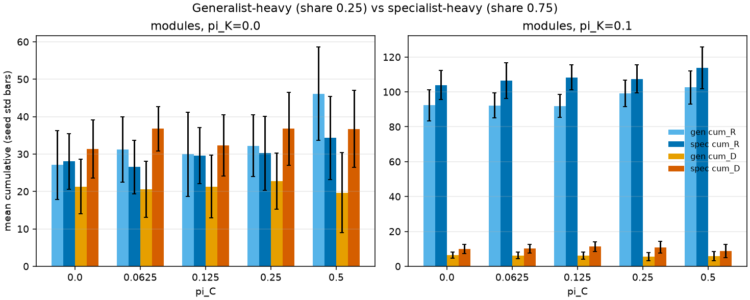
Pre-shock revenue and post-shock discovery are plotted for specialist-heavy and generalist-heavy mixes at each coordinator share.
Promotion is paired on the same seeds, at \(\beta_1 = -1\), with 30 seeds. At the revenue winner, Peter minus Match on post-window revenue is -0.6957 ± 2.0907, and Peter minus Match on post-window mean output is -0.0443 ± 0.0425. At the reference cell, coordinator share 0.125, specialist share 0.5, and communicator share 0.1, Peter minus Match on post-window revenue is -0.6279 ± 0.8513, and on post-window mean output is -0.0355 ± 8.4937e-03.
Tournament minus Peter on post-window mean output is 0.0508 ± 0.0265 at the winner and 0.0490 ± 6.6503e-03 at the reference. Tournament’s post-window coordination loss is higher than Peter’s, not lower: 0.0180 ± 0.0173 at the winner and 6.6024e-03 ± 1.0691e-03 at the reference. The prize does not close the gap. It leaves the roles where they were.
Peter still beat the no-promotion control on post-window revenue at the winner. The paired change in revenue is 0.6377 ± 1.7219, and the paired change in discovery is -1.3867 ± 3.2789. That revenue gap is the sign of the mean, and the seed spread is wider than the mean. It is not a claim that Peter lost to doing nothing. The depth rule gives up discovery and still does not match the breadth rule.
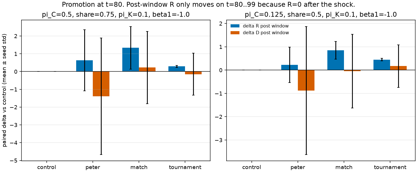
Each promotion rule is shown as its paired change in post-window revenue and discovery against the no-promotion control.
The ranking of coordinator share by cumulative revenue flips once alpha and gamma move. On the modules sweep, specialist share 0.5 and communicator share 0.1, 8 of 9 (alpha, gamma) orders differed from the default order. At alpha 0.5, coordinator share 0.5 was worst. At alpha 2, it was best.
One row is enough to see the size of that flip. At alpha 0.5 and gamma -0.14, cumulative revenue at coordinator share 0.0625 is 194.0200 ± 15.4055, and at coordinator share 0.5 it is 165.6943 ± 10.7996. At alpha 2 and gamma -0.14, coordinator share 0 is 25.4928 ± 1.3317, and coordinator share 0.5 is 43.6735 ± 5.3893. Because that ranking flips with alpha, the coordinator mechanism is not identified.
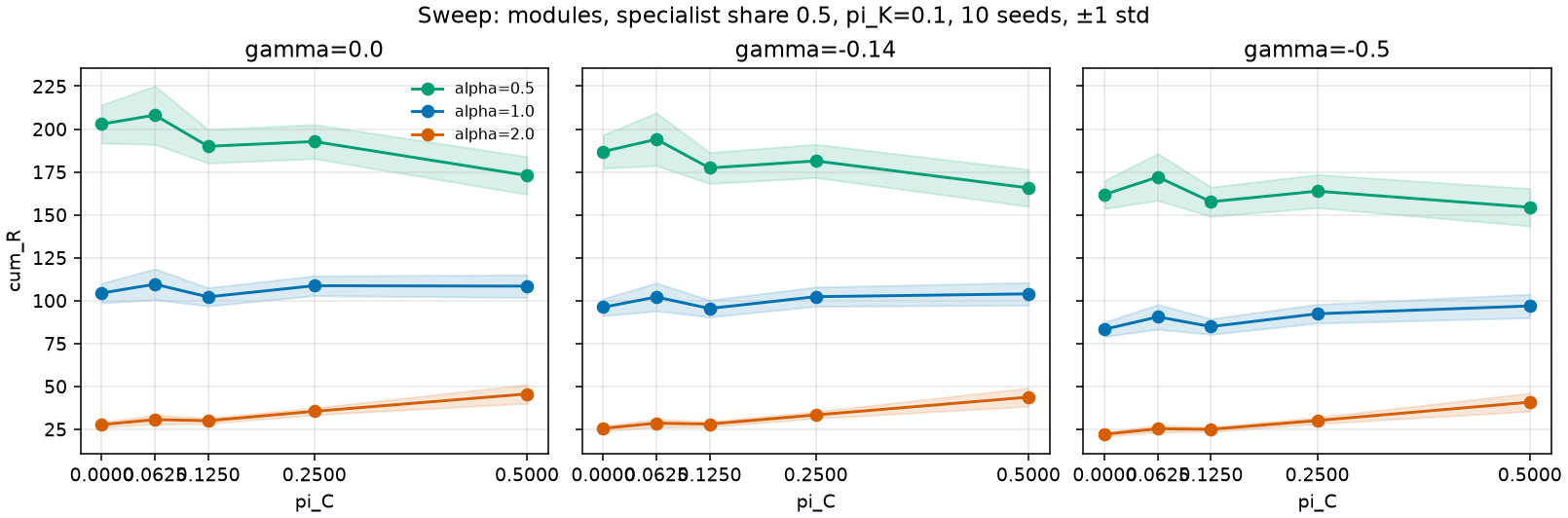
Cumulative revenue is redrawn against coordinator share for each pair of alpha and gamma, on modules only, with 10 seeds.
The sign of Peter minus Match on post-window revenue stayed negative across \(\beta_1 \in \{-1, 0, +1\}\). On the 10-seed winner cell, beta1 of -1 gave -1.0327 ± 2.9471, beta1 of 0 gave -0.8718 ± 4.0372, and beta1 of +1 gave -1.0683 ± 4.1035. Depth entering the new coordination skill with a negative weight, a zero weight, or a positive weight does not turn the comparison around.
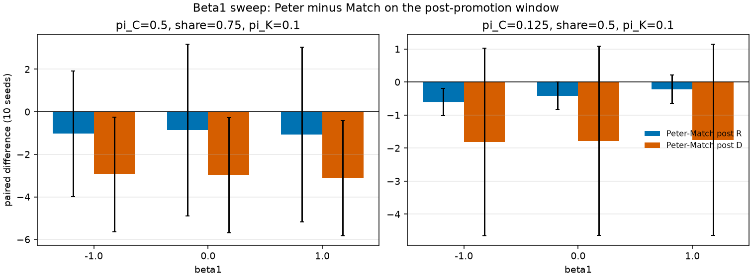
The post-window gap between promoting on depth and promoting on breadth is plotted for revenue and discovery at three values of the depth weight.
A Graicunas sensitivity, not the main loop, replaces the Brooks load inside modules with \(\mathrm{load}(n) = n(2^{n-1}+n-1)\), still times \(\lambda_t\), on 10 seeds. Cumulative revenue is 87.3742 ± 4.5665 at coordinator share 0 and 65.5056 ± 4.9429 at coordinator share 0.5. It is not a clean step down: at 0.0625 the mean is 88.9694 ± 7.0479, above the share-zero cell. This sensitivity swamps the main loop. It is not the main result.
What this does not say
There is no optimal manager percentage for a real company in these numbers. The Greek letters are free parameters. A different alpha reverses which coordinator share wins on revenue.
The too-many-cooks loss in the flat cell showed up as fewer makers, not as a worse coordination gap. Mean effort was higher in the coordinator-heavy flat cell, and the Brooks gap was not worse. Cutting middle management is not supported as a general rule. On this slice the flat group did its best with no coordinators at all, and the modular group did its best revenue with half the group in coordinator roles. Those are two cells in one design.
A firm is not shown to be one mind. The isolated-modules cell, which removes cross-talk by construction, scored higher. That is Simon’s decomposability put in as a switch, not a measured fact about Google or a country.
Questions for a next run
Would heterogeneous socialization speeds change the result? March’s fast and slow learners were not a separate cell here.
What happens if the period has a real task graph, instead of one task per period?
What happens if promotion keeps the maker’s depth, instead of zeroing it?
Is there a prize spread large enough that you can promote on predicted coordination skill and still get the effort? That is Benson’s pay-for-performance margin, and this tournament does not vary the prize.
Would spans that differ by level, wide at the top and narrower in the middle, beat a single coordinator share? That is the shape Cheon reported, and this grid does not try it.